@RISK is used at AMSAA to help senior level officials avoid risks of schedule and cost overruns in equipping and sustaining weapons and materiel for U.S. soldiers in the field.
The US Army Materiel Systems Analysis Activity (AMSAA) conducts critical analyses to provide state-of-the-art analytical solutions to senior level Army and Department of Defense officials. Analyses by AMSAA support the equipping and sustaining of weapons and materiel for U.S. soldiers in the field, and inform plans for the future. @RISK is used at AMSAA to help senior level officials avoid the risks of schedule and cost overruns. New @RISK models integrate schedule and cost consequences, and employ Monte Carlo simulation to give decision-makers the best information possible.
Integrated Model Addresses Schedule and Cost Risks at AMSAA
One of the top priorities of the U.S. Army is to make better decisions in their acquisition programs. When considering any new materiel, decision-makers want to know the risk, cost, performance and operational effectiveness of each new acquisition. In this case, risk is the likelihood of not meeting the target time with schedule and cost consequences.
The US Army Materiel Systems Analysis Activity, known as AMSAA, conducts critical analyses to equip and sustain weapons and materiel for soldiers in the field and future forces. The Army is charged with determining the best possible choice among several acquisition options, taking care to examine alternatives in tradespace, sensitivity, and cost and schedule risk mitigation. Currently, with the help of @RISK, AMSAA conducts separate schedule and technical risk assessments, which are not connected to the cost risk assessment (approaches are in silo). However, AMSAA Mathematician and Statistician John Nierwinski decided to use @RISK to integrate schedule and cost consequences in order to provide a single risk rating that decision-makers can efficiently use to inform the overall decision. “This is cutting edge stuff,” says Nierwinski. Discussions are in process on ways to implement this in the future and gradually phasing out of the silo approach to risk evaluation. This modeling approach has not yet been applied to any acquisition studies; however, some of its submodels have been applied. Integrated risk ultimately translates to integrated schedule and cost that can be traded off with performance and operational effectiveness.
Monte Carlo Simulation Exposes the Risk of Project Overruns
The first step in Nierwinski’s analysis requires a schedule network model, with technology development, integration, manufacturing, and other events. Completion time for these events are assessed using data or subject matter experts (SME). If SME’s are used it is common to use a triangular time distribution with a minimum, maximum and most likely number of months to progress from Milestone (MS) B to MS C. @RISK uses this schedule network model as the main driver of the Monte Carlo process, which is an integrated risk model. For each iteration output of the @RISK model, a consequence determination is made using cost and schedule if the time exceeded the MS C target date. A cost model is used based on the technology cost information that is available. The main cost items are due to the fact that schedule delays can increase variable costs, such as labor expenses. Acquisition variable costs are typically estimated from database or expert information. Hence, if a program goes over the milestone date by a number of months, then the additional cost to the project will be the number of months times the variable cost per month.
With schedule and cost variables in place Nierwinski then creates integrated outputs from the model, which will then, with several thousand iterations, create scenarios that involve an overrun or underrun, depending on the iteration. For overrun situations there are two sets of consequences, cost and schedule. Each set of consequences range from 1-5 (best-case to worst-case scenarios). A given simulated run will yield a cost and a schedule consequence. The maximum of the two consequences is selected for each simulated run. This is called the max consequence. If the target time is not exceeded for a given simulated run, then the max consequence is set to none or 0.
AMSAA Mathematician and Statistician
Getting a Single Risk Rating
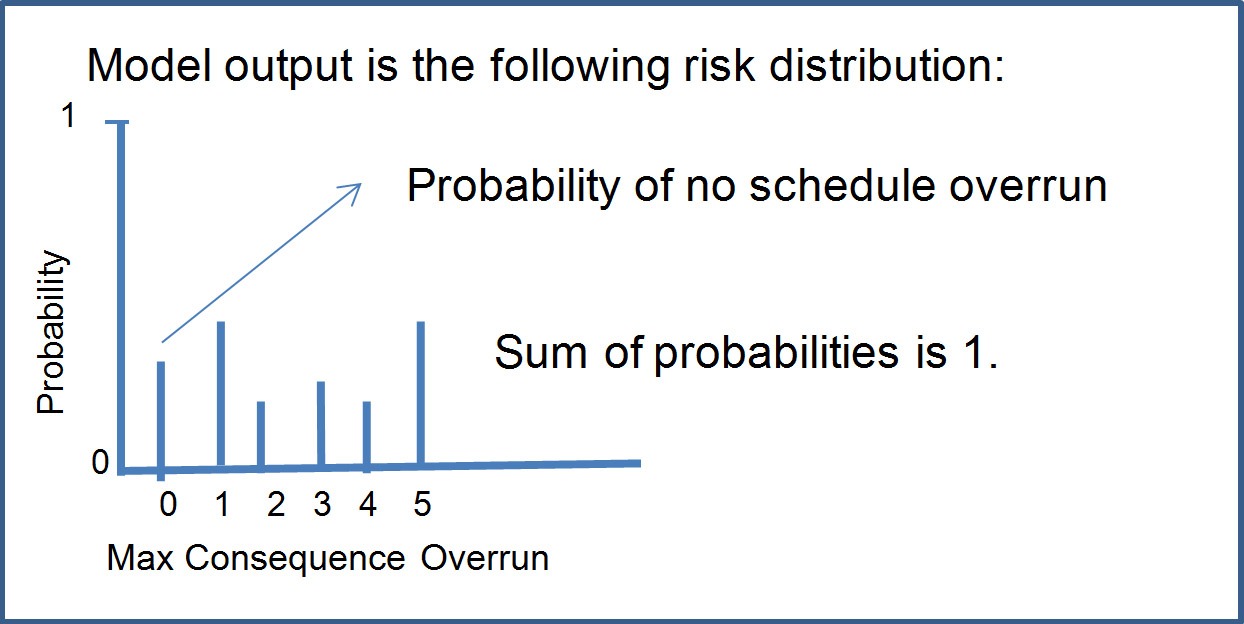
After running the integrated model, @RISK gives an output that tells the likelihood of not meeting the schedule, and the collection of maximum consequences from schedule overrun scenarios.
As the figure above indicates, ‘0’, is the chance that there will be no schedule overrun. Nierwinksi then translates this finding into a matrix to view the risk distribution in table form:

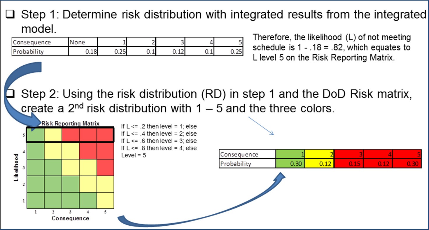
“This allows you to see your probabilities of being in each of these consequence ‘buckets’,” says Nierwinksi. Because this data is a probability distribution, it is easy to determine the probability of not meeting the schedule on time by subtracting the probability of meeting the milestone from 1, (1 – 0.18= 0.82) meaning there is an 82% likelihood of missing the schedule date.
Color-Coding Risk
Nierwinski then applies this distribution to a pre-established DOD color-coding system known as the DOD risk reporting matrix to determine the transformed risk distribution in the lower right hand corner of the figure below. The risk reporting matrix is typically used to report a risk level within a program. The level of risk is reported as low (green), moderate (yellow), or high (red) based on the mapping of the likelihood and consequence to a single square on the risk reporting matrix.

To compute probabilities in the transformed risk distribution, Nierwinski divides probabilities for consequence 1–5 by the probability of missing the schedule date, 0.82 (for example, consequence 1 = .25 / .82 = .30). The transformed consequence level probability is the conditional probability of the consequence level given a schedule overrun. The likelihood of 0.82 corresponds to a likelihood level of 5 in the risk reporting matrix (see figure above) therefore colors are green, yellow, red, red, and red for each consequence. Once Nierwinski formats the risk distribution, he determines an expected color by multiplying the probability of obtaining each color by 1, 2 or 3 (numerical rating: green = 1, yellow = 2, and red = 3). The expected color rating in the example above is:
1(.304) + 2(.12) + 3(.15 + .12 + .302) = 2.27
Next, he transforms the discrete scale of green/yellow/red colors to a continuous numerical scale. Since colors range from green (1) to red (3), the numerical difference is 2. Therefore, a range of 1 to [1 + 2/3 = 1.667] is green; a range of 1.667 to [1.667 + 2/3 = 2.333] is yellow; and 2.333 to 3 is red. Therefore, in our example, a 2.27 rating implies a yellow or medium risk rating for the alternative.
@RISK Brings Flexibility to Modeling Material Acquisitions at AMSAA
“Once we’ve established a risk rating for a certain materiel option, let’s say it’s a particular alternative for a kind of tank, we can do all sorts of studies (i.e. tradespace, what-if scenarios, risk mitigations)—we can examine what would happen to the risk if we were to swap out its engine for a cheaper one,” says Nierwinski. “This can change a lot of things. We can study how the risk rating changes: for example, it may go from high risk to low risk.”
Furthermore, we can extrapolate risk into integrated cost and schedule output, make joint probability statements, and conduct tradeoff decisions with performance and operational effectiveness. @RISK informs this acquisition decision making process.
Nierwinski says that @RISK was instrumental in modeling the inherent risk and uncertainty with materiel acquisitions that AMSAA faces. “@RISK enables us to build various kinds of risk models quickly, with lots of flexibilities.”

