Continuing with this series of articles introducing cost estimating with @RISK, we will compare the use of the most popular distributions of this technique: the Triangular and the PERT.
We know that cost estimation is one of the most critical parts of project management. In addition, we know that three-point estimation – with PERT or triangular distributions – is widely used in this endeavor, but we need to point out that these distributions have different characteristics. The purpose of the following lines is to present them and provide an informed opinion of their use in estimating.
How do three-point estimates work?
Three-point estimating is a simple but useful approach to estimating the cost of the elements of a budget.
There are three different values that are typically obtained from suppliers (from their quotes) and/or from an expert's judgment:
• Optimistic estimate or best-case scenario (lowest cost in this case).
• Pessimistic estimate or worst-case scenario (higher cost in this case).
• Most likely estimate or most realistic scenario
For example, we can have a development task that if everything goes fairly well and we do not have any serious impediment, then the task will last 5 weeks.
However, if we have problems with the code, we could see the construction of the software stretch to up to 10 weeks. On the other hand, if we manage to elaborate this part quickly, we can overlap tasks and conclude the project in 4 weeks.
Therefore the 3 points of the estimation would be:
P = 10 weeks
Ml = 5 weeks
O = 4 weeks
A three-point estimate can be represented by a distribution like the triangular and PERT which belong to this family of continuous probability distributions defined by the minimum (a), most probable (b) and maximum (c) values that a variable can take.
Let's see below a Triangular distribution and a PERT distribution:
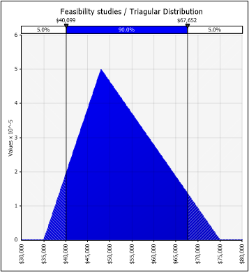
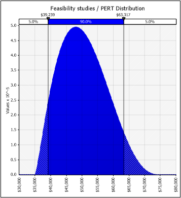
The PERT method allows us to convert the three-point estimate into a smoother curve by assimilating a Normal. When the distribution is skewed, the PERT distribution provides a more "natural" shape than the corresponding Triangular distribution.
The Triangular main drawback is its unnatural shape, which rarely, if ever, describes a natural process adequately. In comparison to the PERT distribution, it tends to overestimate the tails and underestimate the shoulders.
Let's see a comparison between the Triangular and a PERT distribution:
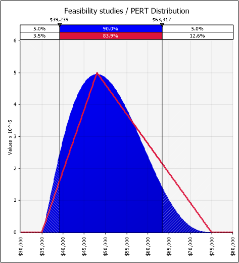
Considering the above, using the triangular method is recommended when there is no history of similar projects, as there is no basis for giving a particular estimate more weight. Therefore, the triangular distribution is more suitable for expert judgment estimates or rather guess estimates.
Note: Comparative analysis of two or more distributions can be done using the overlays’ function offered by @RISK in the distributions panel.
An example in @RISK
Continuing with the example of the previous article, we will explore the use of distributions in a cost and contingency model.
In this case we are going to add two columns with the estimates represented with the Triangular and the PERT:

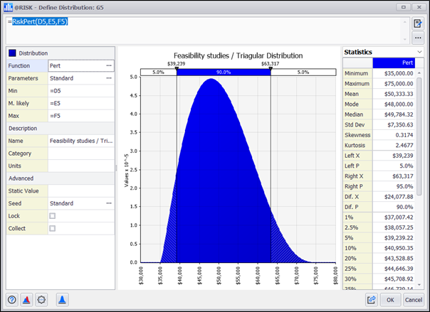
We can now configure each cost element using the @RISK functions to design the distributions:
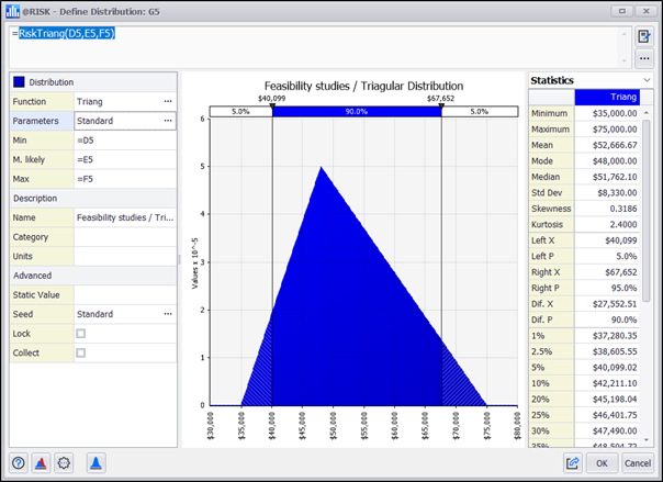
The next step is to complete all cost elements with the corresponding formulas:

We sum each of the columns to have all the deterministic and probabilistic scenarios in order. We then declare the totals of the probabilistic columns as outputs of the Monte Carlo simulation model:

![]()
We are now ready to run the simulation. Let's test with 1000 iterations and see the effects on the results:

This process will take a few seconds in @RISK and will generate 1000 independent combinations of our cost items and their corresponding results:
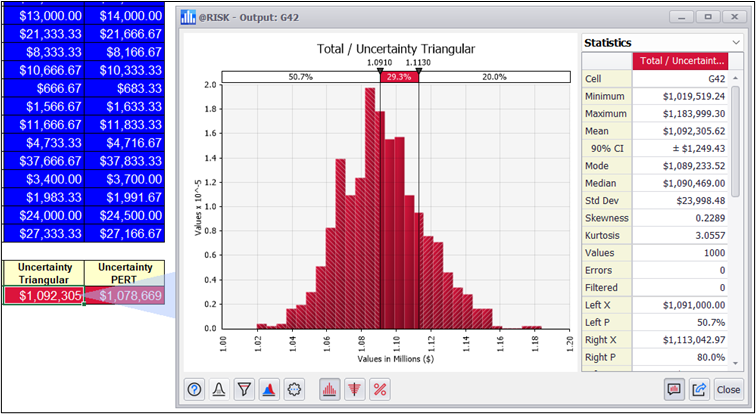
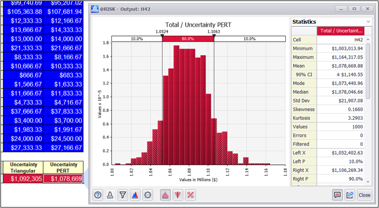
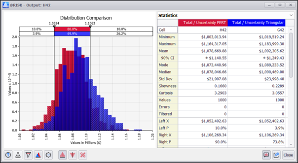
The distributions of results are similar, but if we look at their descriptive statistics, there are some differences to consider:
Conclusion
Three-point analysis can benefit from the PERT distribution as an alternative to the triangular distribution. One advantage of the PERT is that it has a smoother shape than a triangular distribution, with an emphasis on the most probable value. Although we are interested in the mathematics of the triangular distribution when we are unsure of the weights given to the expert criteria.
The correct selection and combination of the distributions, facilitated by the simple use of @RISK, allows us a more justifiable and solid analysis for our decision-making when cost estimating.
Try this for yourself by downloading your 15-day free trial of @RISK.
Originally Published: Nov. 1, 2022
Updated: Sept. 1, 2023
At the time of this article's publication in November 2022, the U.S. dollar was at its highest level since 2000, up more than 20 percent over other major currencies such as the British pound, the euro, and the yen. The economic forecast was for more volatility in 2023, which tends to drive further demand for the dollar, seen as a safe harbor investment during periods of uncertainty. However, as we’ve seen with the rapid depreciation of major currencies this year, this could change at any moment. It’s important to account for variability and uncertainty in exchange rates as part of the treasury planning process heading into next year.
The strong dollar means potentially significant losses for US firms who transact in foreign currencies. When those sums are eventually converted back to dollars, their value will be substantially reduced. Short of simply transacting exclusively in US dollars – an unrealistic prospect for most international firms – the most common tactic for mitigating such foreign currency risk is to hedge against future movements in the value of the currency. This can take the form of options, which give the holder the right (but not the obligation) to buy or sell an asset such as a currency at a specified price, or of forward contracts, which obligate the holder to buy or sell an asset at a given price.
In order to determine the best hedging strategy, a sophisticated understanding of likely future movements of currency prices is needed. Monte Carlo simulation fits this bill very well, providing a view into hundreds or thousands of possible future outcomes, with or without a hedging strategy in place. Furthermore, simulation of time-series variables – or factors that move over time, such as exchange rates – is critical. In addition, Monte Carlo can be performed on multiple hedging strategies, enabling decision-makers to identify the optimal strategy to meet their goals within their specific risk tolerances.
The model linked below provides a simple example of how a hedging strategy – the purchase of put options, which give the holder the right to sell a currency at a given price – can significantly improve the likelihood of better outcomes in today’s foreign exchange environment. The model uses @RISK Industrial to run the analysis, which includes advanced functions for modeling time-series variables.
Download the Example Model: Exchange Rate Hedging
This article offers a simple and concise explanation of the Monte Carlo simulation, a technique that combines statistical concepts (random sampling) with the ability of computers to generate pseudo-random numbers and automate calculations, for basic cost engineering.
The key to Monte Carlo simulation is to create a mathematical model of the system, process, or activity to be analyzed – identifying those variables (model inputs) whose random behavior determines the overall behavior of the system. Once these inputs or random variables have been identified, an experiment is carried out which consists of generating random samples (specific values) for these inputs and analyzing the behavior of the system in response to the values generated. After repeating this experiment ‘n’ number of times, we will have ‘n’ number of observations on the behavior of the system, which will be useful to understand how the system works.
Let us look at an example of a Monte Carlo simulation cost model with continuous random variables where the model will assume we are calculating the contingency reserves for a temporary COVID-19 hospital construction project. These temporary projects have the same cost structure, but the values change from region to region. Because of variability, engineers must do a contingency analysis for each project. Typically, a percentage of the total will be used as a contingency, and we will try to improve this approach.
To infer the distributions of each cost element, historical data is ideal. However, in this type of application, there is typically not enough data for an automated fit. Therefore we will use expert judgment or the results of analyzing suppliers' bids to construct the input distributions.
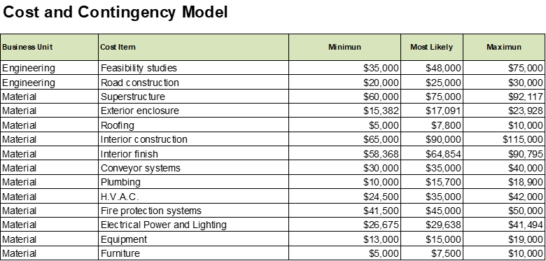
The following image shows a partial list of the cost elements in the example, each with a minimum, most probable, and maximum value. This data can be used to set up three-point distributions which are the most popular in cost engineering.
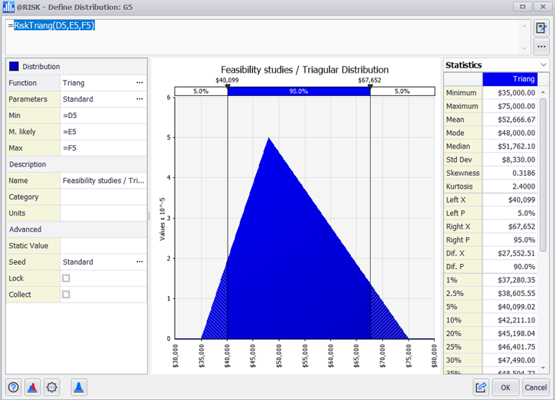
The next step is to add a column to set up a probability distribution for each cost element. After selecting the Triangular distribution and setting its three parameters: minimum, most likely, and maximum, we would get a correctly designed distribution. To improve the fit of the distribution, we can change alternative parameters such as the static value in the Excel cell (otherwise it will use the mean) or specialized parameters.
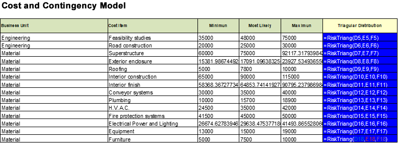
We can copy and paste the distribution formula into the cells of all the cost elements with uncertainty and verify that the formula parameters are set correctly.
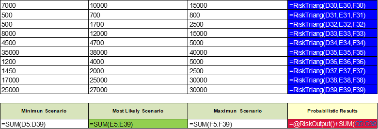
A total budget will be generated by adding up all distributions and declaring it as the Monte Carlo simulation model's output. This requires selecting the output menu and setting the name.
Now that we are ready to run the simulation, let's use 1000 iterations in this first test.

Once the process is finished, @RISK makes the results available with graphs, such as a histogram, and we can compare the original most probable budget against our expected value from the probabilistic model.
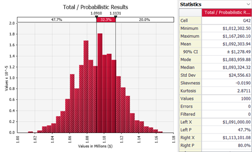
It is recommended to use the concepts of Expected Value (mean of the simulation results) and the percentile with the risk level established by the company's PMO policies, in this case the 80% percentile. The difference between the P80 and the Expected Value would give us the value of the PMO contingency reserve.

Evidently, we can see a more interesting and justifiable technique for the calculation of contingencies; although we need to also consider that in this model, we have not considered the effect of unplanned risk events and we have reduced the model to a single distribution (Triangular).
Future articles will explain how it is possible to extend the cost engineering model by comparing it with other similar distributions or by adding a risk register that considers low probability and high impact events.
Explore @RISK by downloading a 15-day free trial.