


In our previous article, Introduction to Lean Six Sigma, we discussed the fundamentals of Lean Six Sigma, exploring how it combines the principles of lean manufacturing and Six Sigma to drive process improvement and operational excellence.
Now, we’re taking the next step by diving into how risk analysis software, specifically with Lumivero’s @RISK software, can enhance Lean Six Sigma initiatives. This post will focus on how Monte Carlo simulation can empower organizations to predict, manage, and mitigate risks, ensuring the success of Lean Six Sigma projects by drawing from insights shared in François Momal’s webinar series, “Monte Carlo Simulation: A Powerful Tool for Lean Six Sigma” and “Stochastic Optimization for Six Sigma.”
Together, we’ll explore real-world examples of how simulation can optimize production rates, reduce waste, and foster data-driven decision-making for sustainable improvements.
Monte Carlo simulation, as a reminder, is a statistical modeling method that involves making thousands of simulations of a process using random variables to determine the most probable outcomes.
Model 1: Predicting Process Lead Time as Seen by Customers
The first model Momal presented involved predicting the lead time for a manufacturing process. He described the question this model could answer as, “when I give a fixed value for my process performance to an internal or external customer, what is the associated risk I take?”
Using data on lead time for each step of a six-step production process, @RISK ran thousands of simulations to determine a probable range for the lead time. It produced three outputs:\
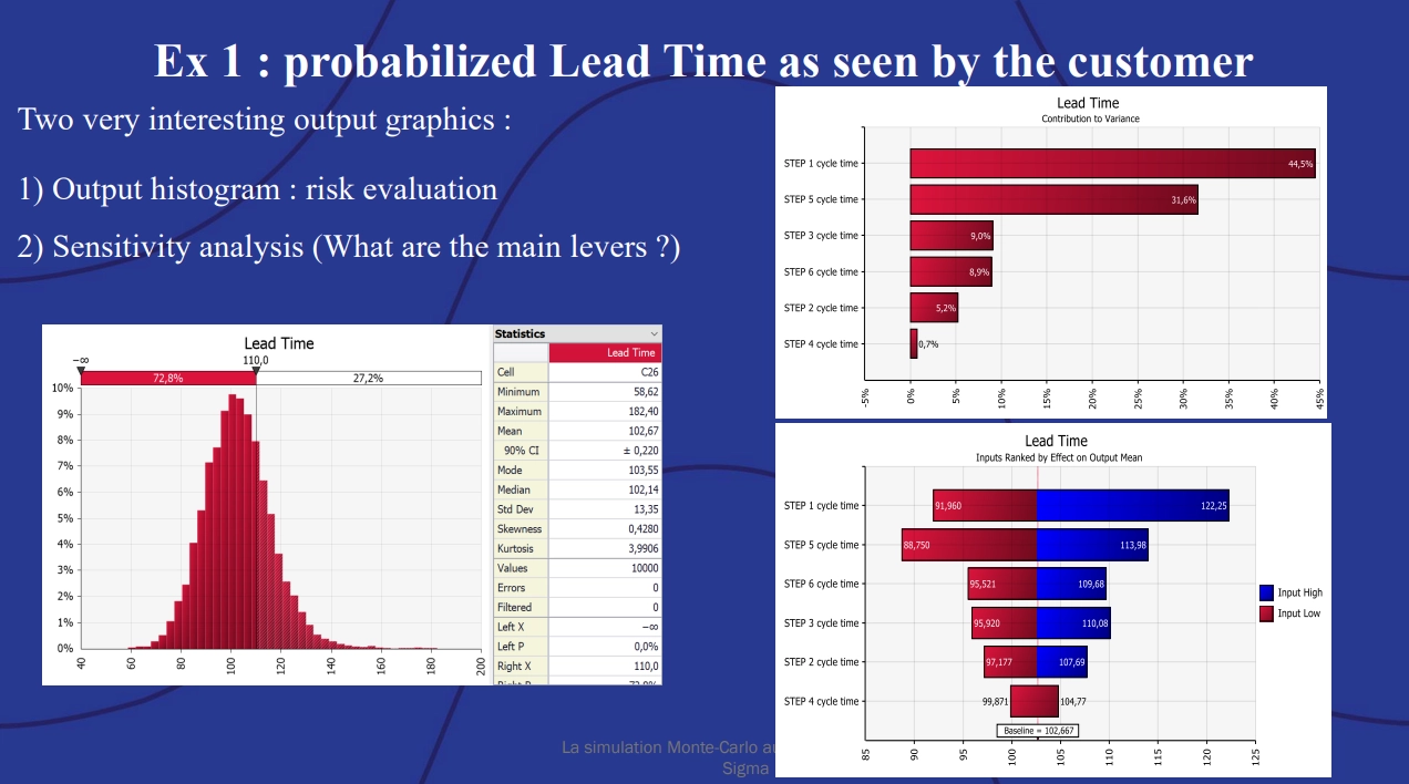
Example 1: Probable lead time as seen by the customer showing two output graphics: output histogram for risk evaluation and sensitivity analysis showing what the main levers are.
The left-hand chart shows the probability distribution curve for the lead time which allows the production manager to give their customer an estimate for lead time based on probability. The other two charts help identify which steps to prioritize for improvement. The upper right-hand chart shows which of the six steps contribute most to variation in time, while the lower-right hand chart describes how changes to the different steps could improve that time.
@RISK also allows production managers to set probability-based improvement targets for each step of the process using the Goal Seek function.
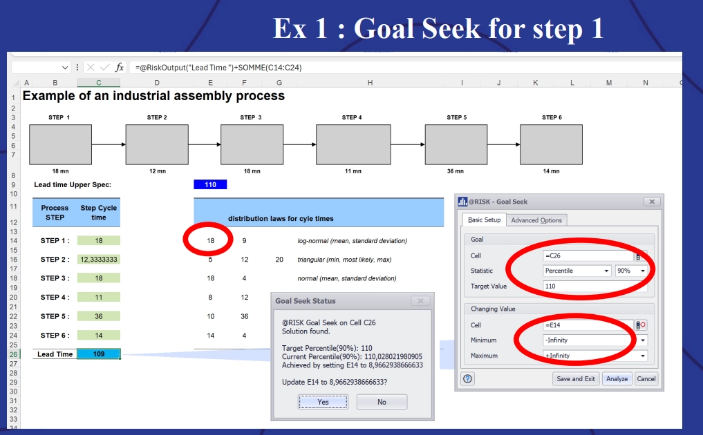
Example 1: Goal Seek for step 1. Example of an industrial assembly process.
Model 2: Value-Stream Mapping and Determining Hourly Production Rate
As mentioned above, the “Lean” aspect of Lean Six Sigma often refers to speed or efficiency of production. Lean production relies on being able to accurately measure and predict the hourly production rates of an assembly line.
Momal’s second example was a model which compared two methods of finding estimated production rates for a five-step manufacturing process: a box plot containing 30 time measurements for each step, and a Monte Carlo simulation based on the same data.
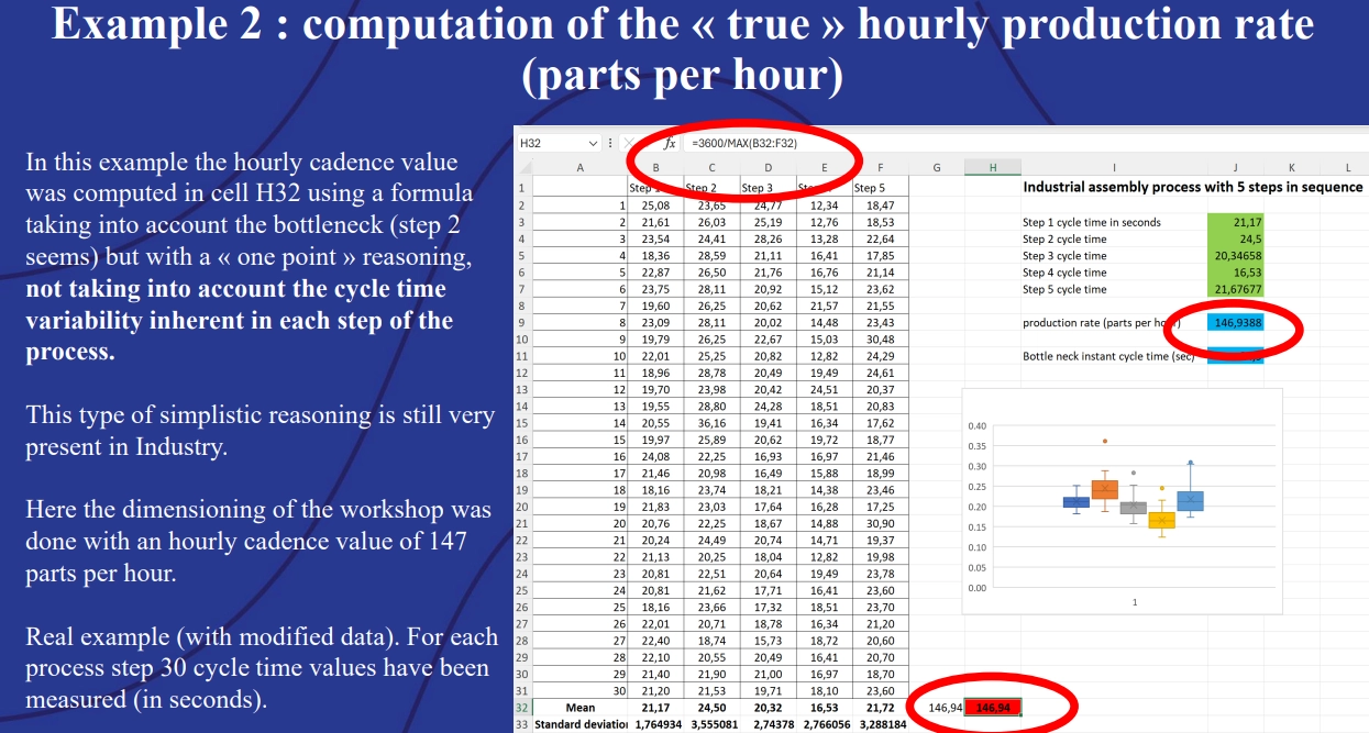
Example 2: Computation of the true hourly production rate (parts per hour).
Both the box plot and the Monte Carlo simulation accounted for the fact that step two of the production process was often slower than the others – a bottleneck. However, the box plot only calculated the mean value of the time measurements, arriving at a production rate of approximately 147 units per hour. This calculation did not account for variability within the process.
Using @RISK to apply Monte Carlo simulation to the model accounts for this variance. The resulting histogram shows that the assembly line only achieves a production rate of 147 units per hour in 37.2% of simulations.
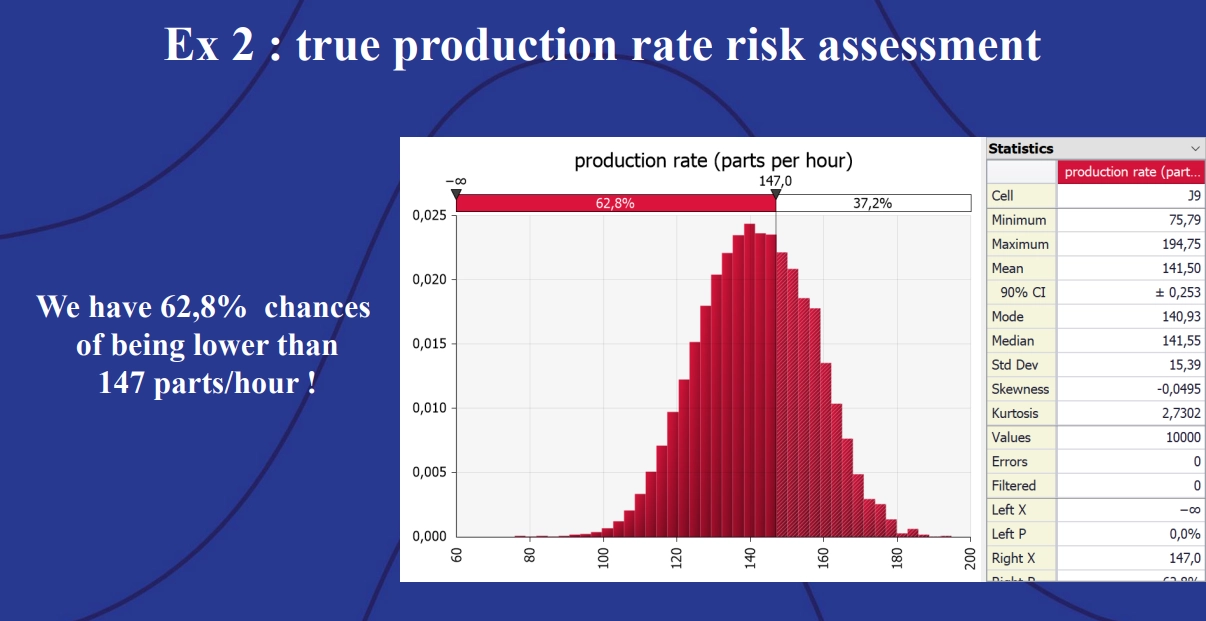
Example 2: True production rate risk assessment.
A plant manager trying to achieve 147 units per hour will be very frustrated, given that there is a 62.8% chance the assembly line will not be able to meet that target. A better estimate for the engineers to give the plant manager would be 121.5 units per hour – the production line drops below this rate in only 10% of simulations:
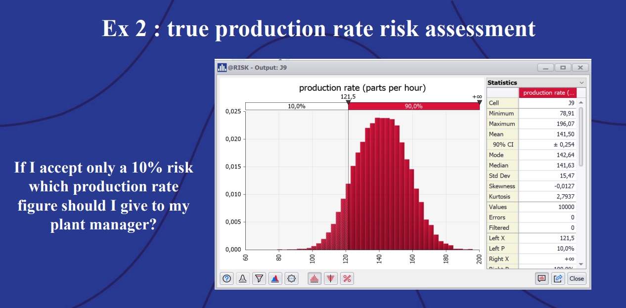
Example 2: True production rate risk assessment, accepting a 10% risk.
Furthermore, with the Monte Carlo simulation, engineers working to optimize the assembly line have a better idea of exactly how much of a bottleneck step two of the process causes, and what performance targets to aim for to reduce its impact on the rest of the process. “The whole point with a Monte Carlo simulation,” explained Momal, “is the robustness of the figure you are going to give.”
Model 3: Tolerancing Components with Monte Carlo Simulation
From Lean modeling, Momal moved on to Six Sigma. Monte Carlo simulation can be applied to tolerancing problems – understanding how far a component or process can deviate from its standard measurements and still result in a finished product that meets quality standards while generating a minimum of scrap.
Momal used the example of a piston and cylinder assembly. The piston has five components and the cylinder has two. Based on past manufacturing data, which component is most likely to fall outside standard measurements to the point where the entire assembly has to be scrapped? A Monte Carlo simulation and sensitivity analysis completed with @RISK can help answer this question.
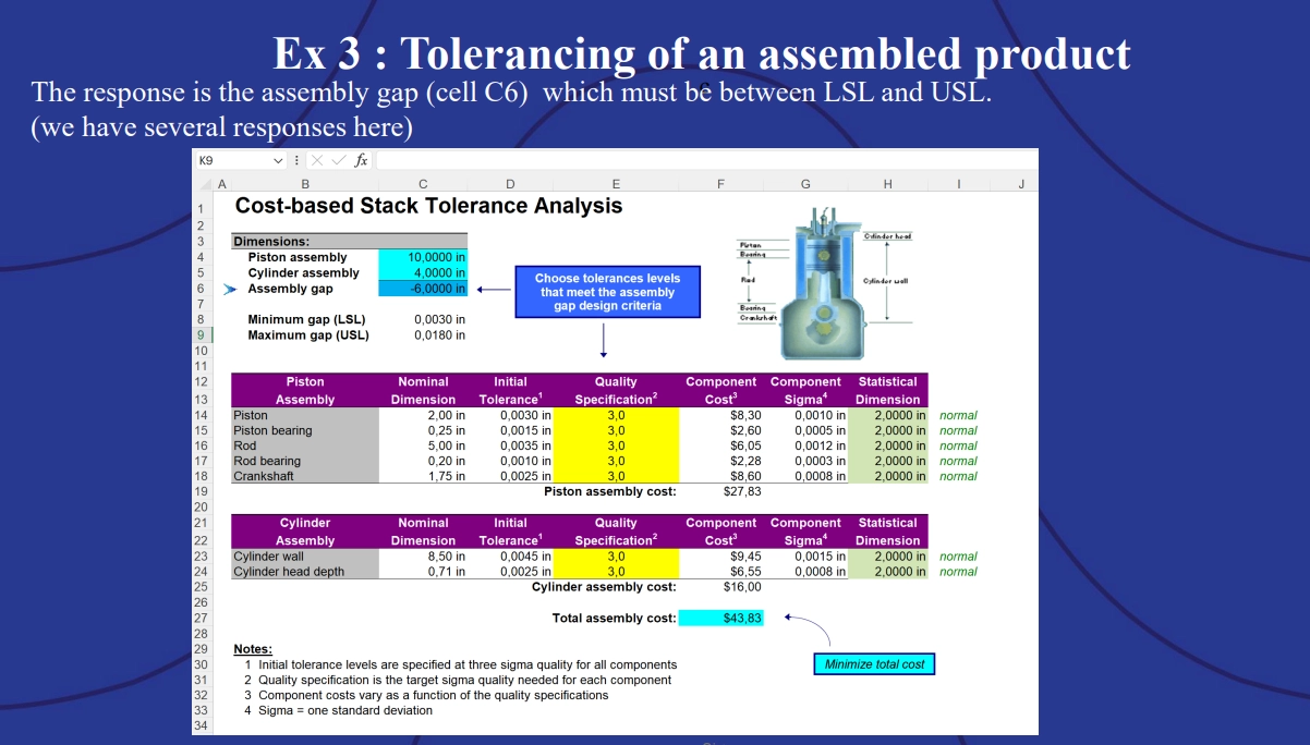
Example 3: Tolerancing of an assembled product, showing a cost-based stack tolerance analysis chart.
In this tolerance analysis, the assembly gap (cell C6) must have a positive value for the product to fall within the acceptable quality range. Using a fixed quality specification, it’s possible to run a Monte Carlo simulation that gives the probability of production meeting the specified assembly gap given certain variables.
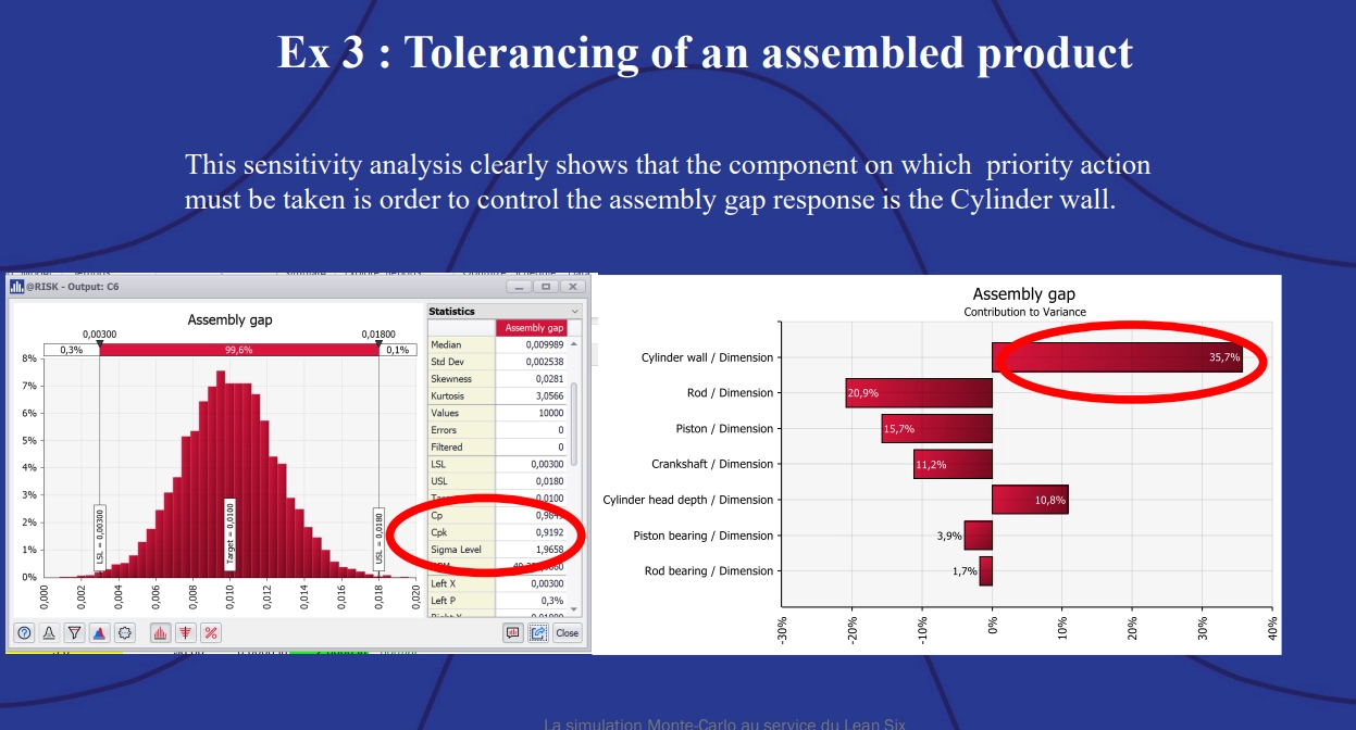
Example 3: Tolerancing of an assembled product, showing sensitivity analysis.
Then, using the sensitivity analysis, engineers can gauge which component contributes the most variation to the assembly gap. The tornado graph on the right clearly shows the cylinder wall is the culprit and should be the focus for improving the quality of this product.
Applying Stochastic Optimization to Support Lean Six Sigma Goals
Stochastic optimization refers to a range of statistical tools that can be used to model situations which involve probable input data rather than fixed input data. Momal gave the example of the traveling salesman problem: suppose you must plan a route for a salesman through five cities. You need the route to be the minimum possible distance that passes through each city only once.
If you know the fixed values of the distances between the various cities, you don’t need to use stochastic optimization. If you’re not certain of the distances between cities, however, and you just have probable ranges for those distances (e.g., due to road traffic, etc.), you’ll need to use a stochastic optimization method since the input values for the variables you need to make your decision aren’t fixed.
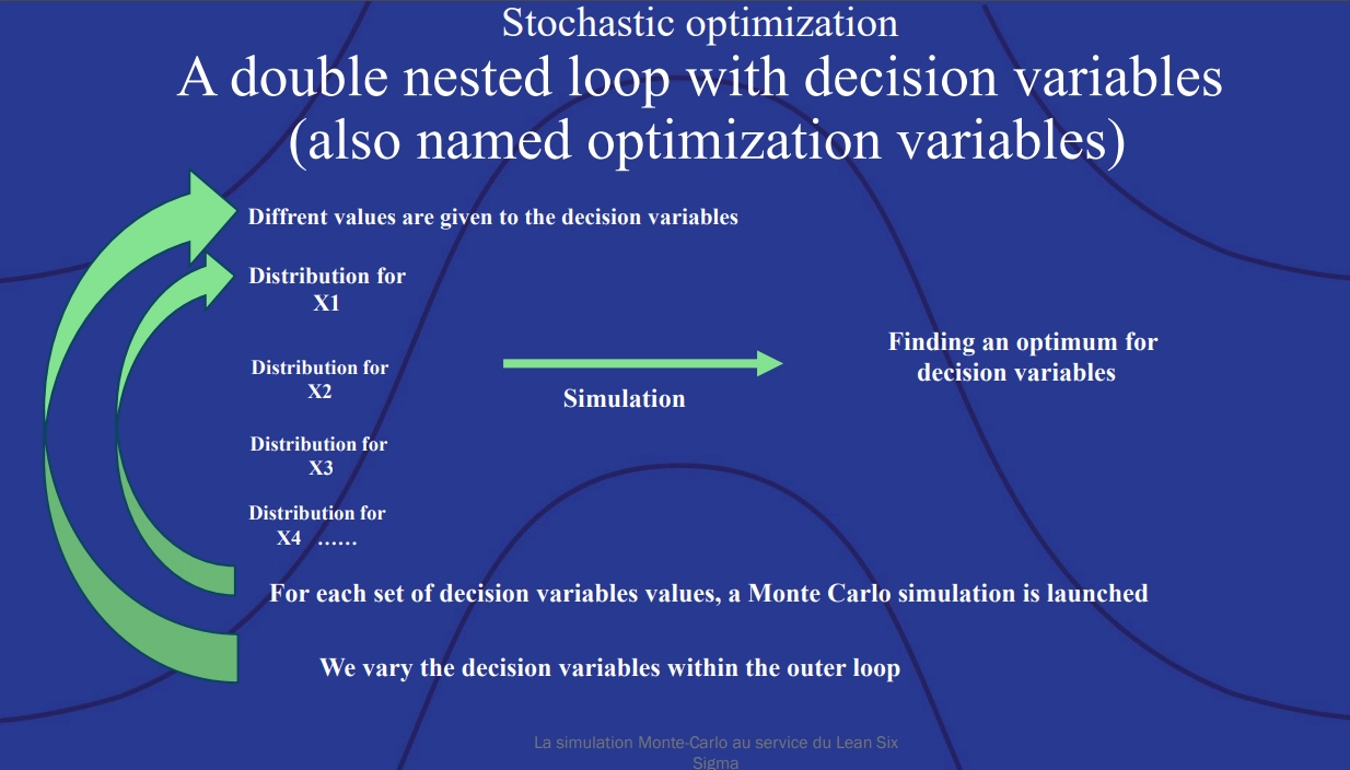
Stochastic optimization: A double nested loop with decision variables (also named optimization variables).
Within the stochastic optimization simulation, a Monte Carlo simulation is completed for each variable within the “inner loop,” and then another Monte Carlo simulation is run across all the variables using different values (the “outer loop”).
Model 4: Prioritizing Six Sigma Project Launches with @RISK Stochastic Optimization
For Lean Six Sigma organizations, stochastic optimization can support better project planning. Momal’s first model showed how to run a stochastic optimization to determine which project completion order would maximize the economic value add (EVA) of projects while minimizing time and labor costs so they remain within budget.
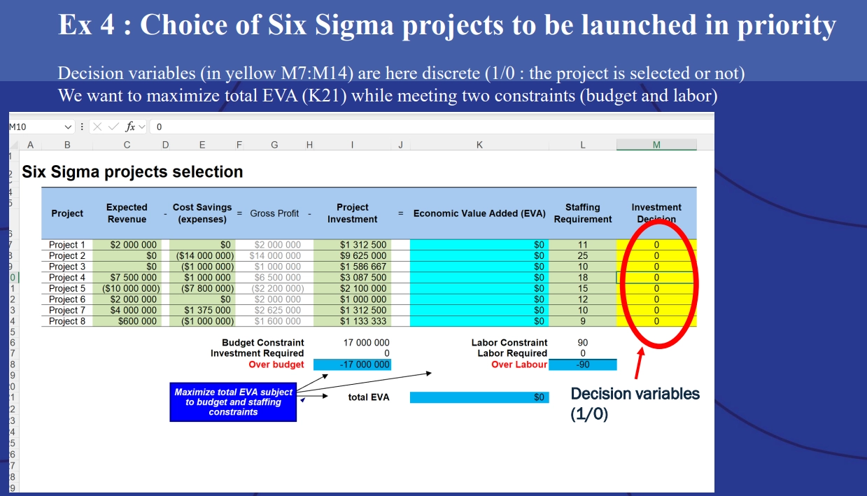
Example 4 Choice of Six Sigma projects to be launched in priority.
To use @RISK Optimizer, users must define their decision variables. In this model, Momal decided on simple binary decision variables. A “1” means the project is completed; a “0” means it isn’t. Users must also define any constraints. Solutions found by the simulation which don’t fit within both constraints are rejected.
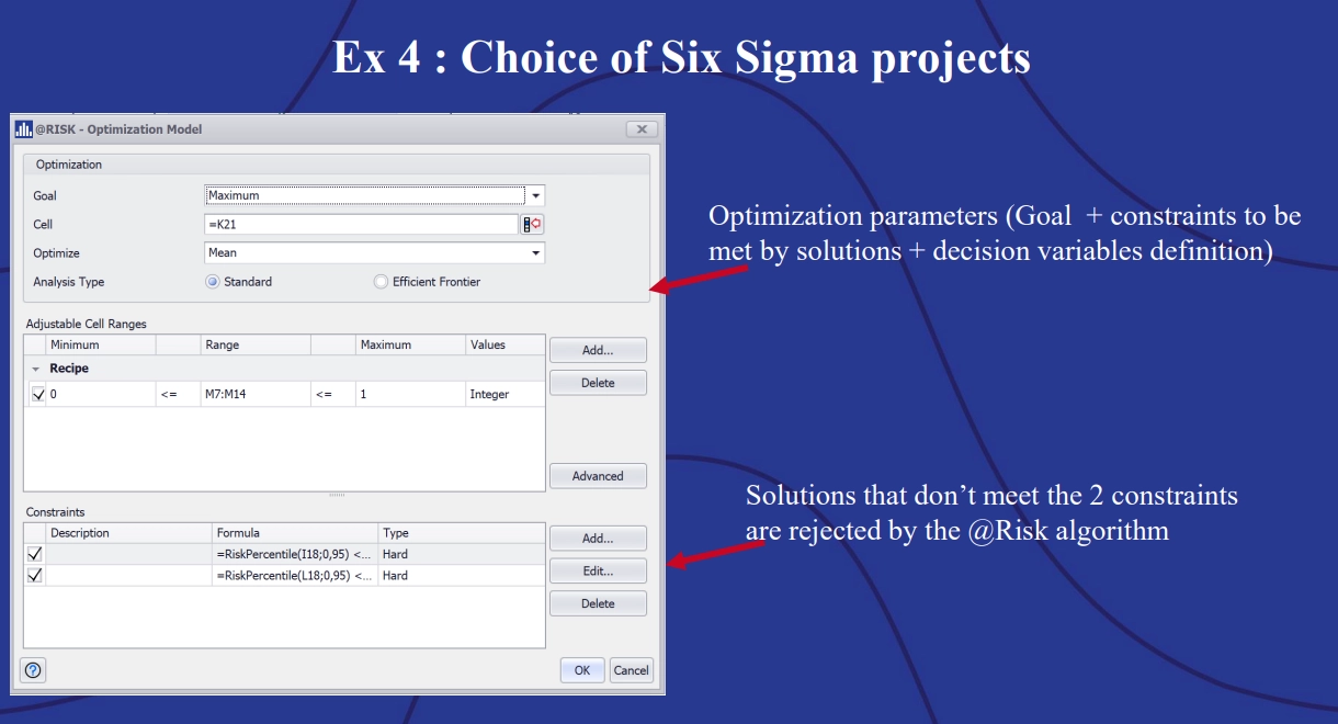
Example 3: Choice of Six Sigma projects, showing optimization parameters and solutions that don’t meet the two constraints.
The optimization was run with the goal of maximizing the EVA. With @RISK, it’s possible to watch the optimization running trials in real time in the progress screen. Once users see the optimization reaching a long plateau, it’s generally a good time to stop the simulation.
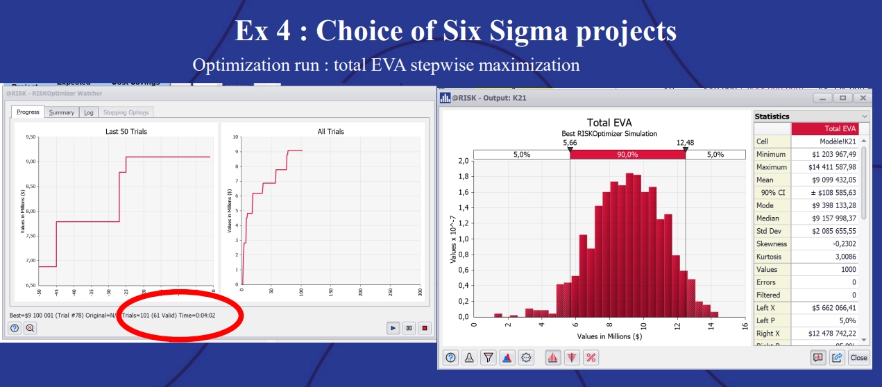
Example 4: Choice of Six Sigma projects showing optimization run: total EVA stepwise maximization.
In this instance, the stochastic optimization ran 101 trials and found that only 61 were valid (that is, met both of the constraints). The best trial came out at a maximum EVA of approximately $9,100,000. The projects selection spreadsheet showed the winning combination of projects:
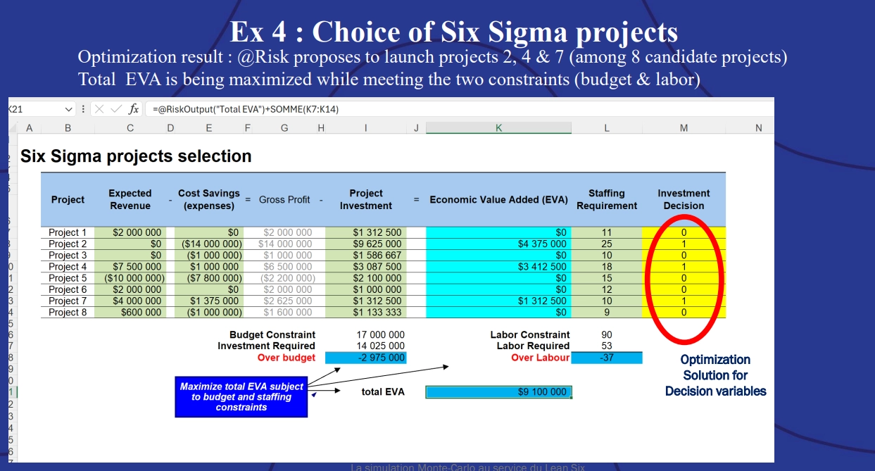
Example 4: Choice of Six Sigma projects optimization results.
Of the eight candidate projects involved, @RISK says that projects 2, 4, and 7 will meet the budget cost and labor time constraints while maximizing the EVA.
Model 5: Informing Pump Design with Design for Six Sigma (DFSS)
Next, Momal showed how stochastic optimization can be applied to design problems – specifically within the Design for Six Sigma (DFSS) methodology. DFSS is an approach to product or process design within Lean Six Sigma. According to a 2024 Villanova University article, the goal of DFSS is to “streamline processes and produce the best products or services with the least amount of defects.”
DFSS follows a set of best practices for designing components to specific standards. These best practices have their own terminology which Six Sigma practitioners must learn, but Momal’s model can be understood without them.
The goal of this demonstration was to design a pump that minimizes manufacturing defects and cost per unit.
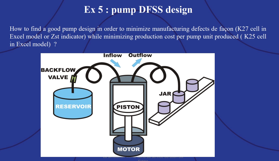
Example 5: Pump DFSS design.
The model used to set up the stochastic optimization included a set of quality tolerances for the flow rate of the pump – this is what is known in DFSS as the “critical to quality” (CTQ) value – the variable that is most important to the customer. Decision variables included motor and backflow component costs from different suppliers as well as the piston radius and stroke rate. The goal was to minimize the unit cost and the quality level of the pump while meeting the flow rate tolerances.
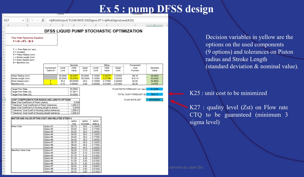
Example 5: Pump DFSS design showing decision variables and tolerances.
As with the previous model, Monal demonstrated how to define the variables and constraints for this model in @RISK.

Example 5: Pump DFSS design, answering the question of “how can we guarantee a certain level of quality?”.
Then, when Monal ran the simulation, he again watched the live progress screen within @RISK to see when a plateau was reached in the results. He stopped the simulation after 1,000 trials.
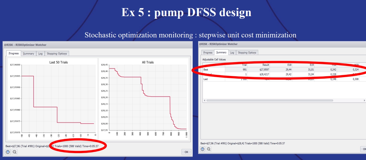
Example 5: Pump DFSS design, showing stochastic optimization monitoring.
The simulation showed that trial #991 had the best result, combining the lowest cost while meeting the CTQ tolerances. Finally, @RISK updated the initial stochastic optimization screen to show the best options for supplier components.
Model 6: Using @RISK and XLSTAT to Improve Design of Experiments (DOE) in Six Sigma
Experiments are necessary in manufacturing, but they are expensive. Six Sigma methodology includes best practices for design of experiments (DOE) that aims at minimizing the cost of experiments while maximizing the amount of information that can be gleaned from them. Monal’s final model used XLSTAT to help design experiments which would solve an issue with a mold injection process that was causing too many defects – the length of the part created should have been 63 mm.
The approach involved running a DOE calculation in XLSTAT followed by a stochastic optimization in @RISK. There were three known variables in the injection molding process: the temperature of the mold, the number of seconds the injection molding took (cycle time), and the holding pressure. He also identified two levels for each variable: an upper level and a lower level.
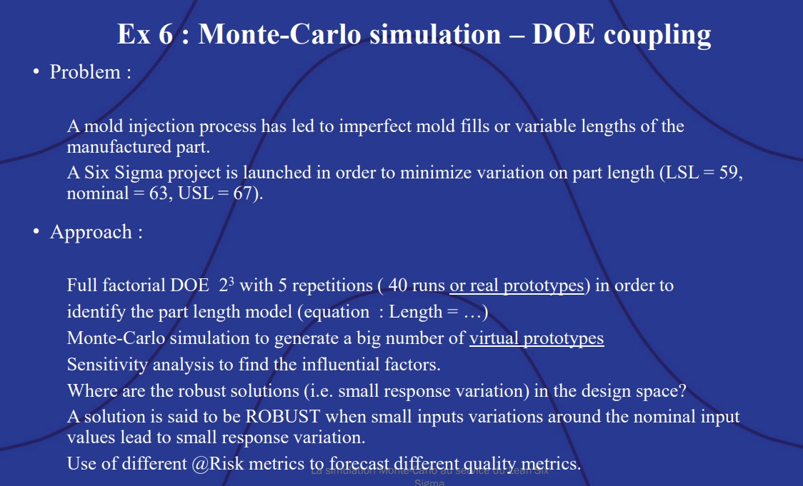
Example 6: Monte Carlo simulation – DOE coupling.
Six Sigma DOE best practices determine the number of prototype-runs an experiment should attempt by taking the number of levels for the variables, then raising them to the power of the overall number of variables, and finally multiplying that value by five. In this instance, 23 is equal to 8, and 8 x 5 is 40. There should be 40 real prototypes generated. These were modeled with XLSTAT DOE. The “response 1” value shows the length of the part created.
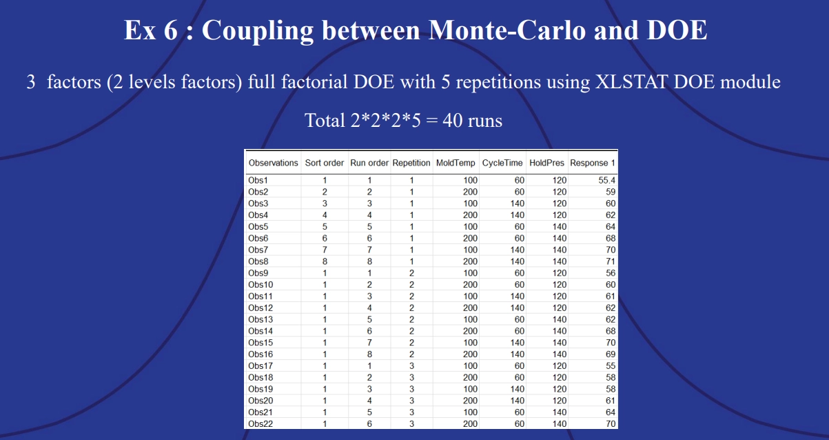
Example 6: Coupling between Monte Carlo and DOE.
XLSTAT then generated a list of solutions – combinations of the three variables that would result in the desired part length. The row circled in red had the lowest cycle time. It also created a formula for finding these best-fit solutions.
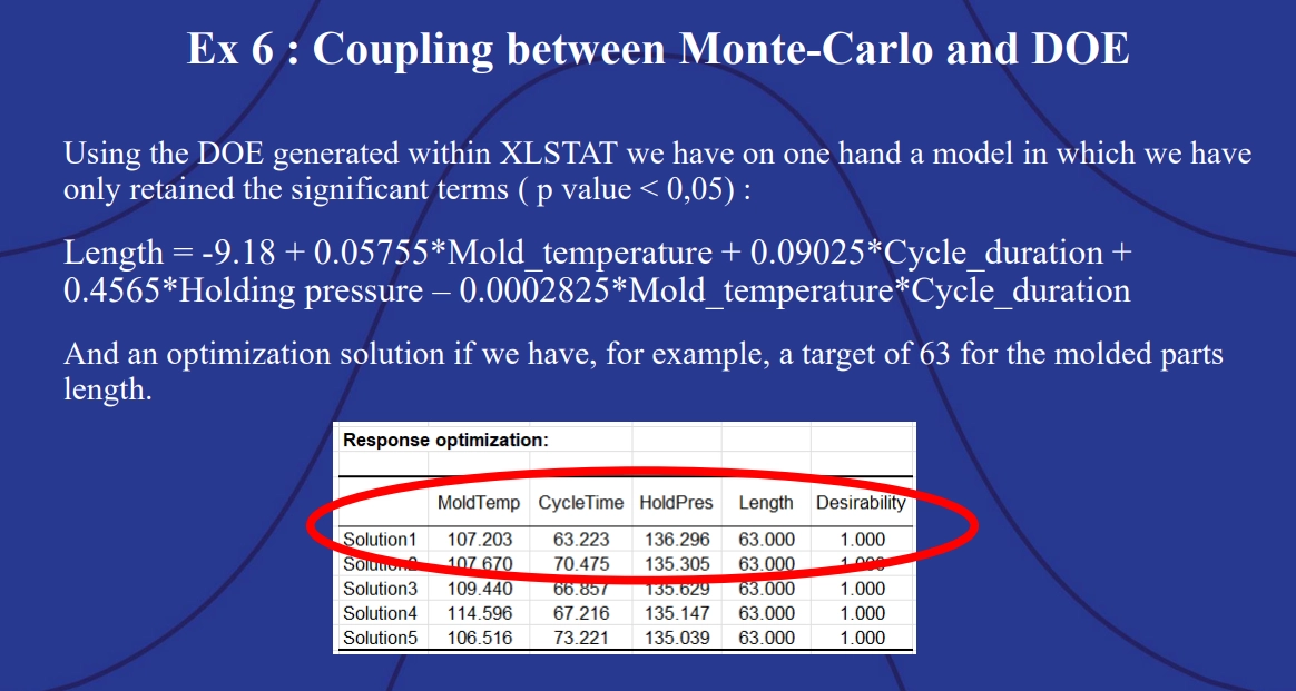
Example 6: Coupling between Monte Carlo and DOE.
These were all possible solutions, but were they robust solutions? That is, would a small variation in the input variables result in a tolerably small change in the length of the part created by the injection molding process, or would variations lead to unacceptable parts?
For this second part of the process, Momal went back to @RISK Optimizer. He defined his variables and his constraint (in this case, a part length of 63). He used the transfer function generated by the XLSTAT DOE run.
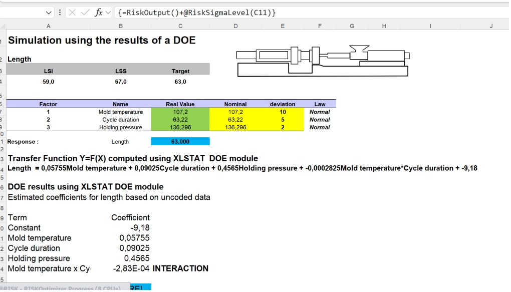
Simulation using the results of a DOE.
Next, he specified that any trials which resulted in a variation of more than three standard deviations (three sigma) in the variables or the length of the part should be rejected.
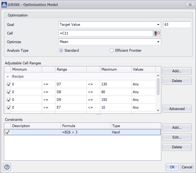
@RISK optimization model set up.
Then he ran the stochastic optimization simulations and watched the outputs in real time.
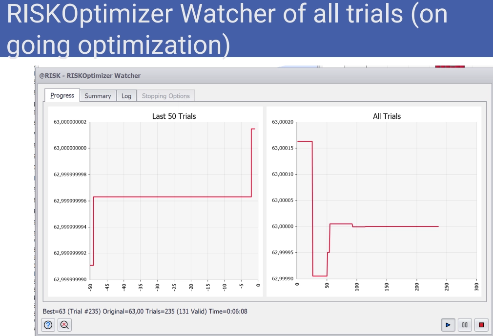
RISKOptimizer Watcher of all Trials (ongoing optimization).
He stopped the trials once a plateau emerged. @RISK Optimizer automatically placed the values from the best trial into his initial workbook.
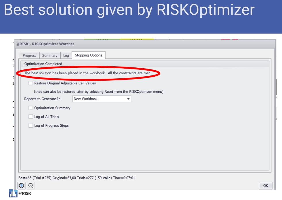
Best solution given by RISKOptimizer.
Sensitivity analysis, this time using a Pareto chart instead of a tornado graph, showed that the primary factor driving variance in trial results was the hold pressure:
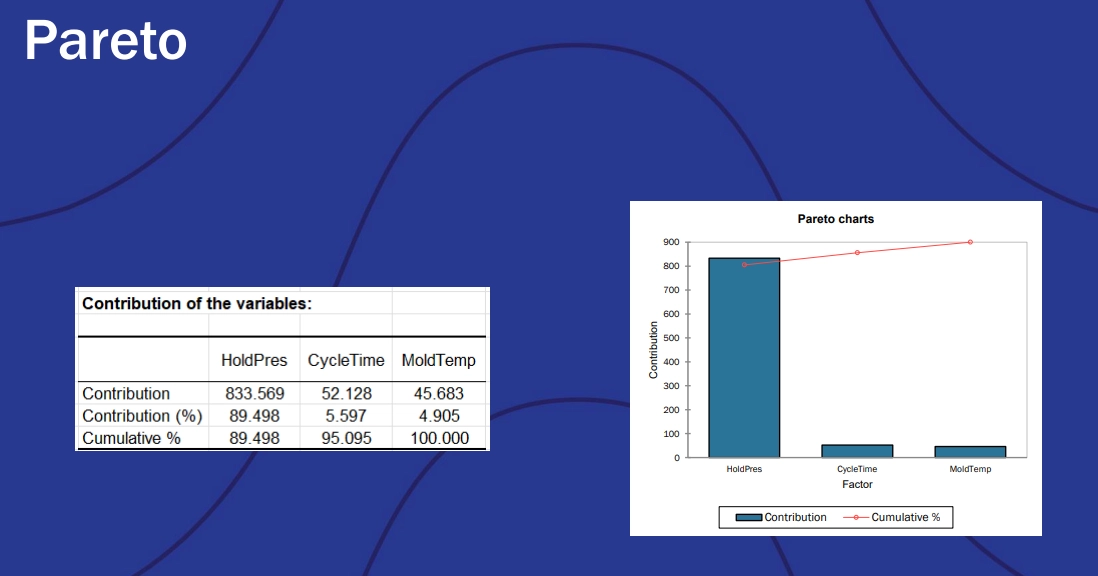
Pareto chart examples including the contribution of the variables.
This gave him experimental data that could be used to inform the manufacturing process without the cost of having to run real-world experiments.
Power Your Lean Six Sigma Strategy with @RISK and XLSTAT
Data-driven manufacturing processes that lead to better efficiency, less waste, and fewer defects – that’s the power of the Lean Six Sigma approach. With @RISK and XLSTAT, you gain a robust suite of tools for helping you make decisions that align with Lean Six Sigma principles.
From better estimates of production line rates to designing experiments to solve manufacturing defect problems, the Monte Carlo simulation and stochastic optimization functions available within @RISK and XLSTAT can support your efforts toward continuous improvement.
Ready to find out what else is possible with @RISK? Request a demo today.


