


Dr. Etti Baranoff, an Associate Professor of Insurance and Finance at Virginia Commonwealth University in Richmond uses @RISK in her business school class, ‘Managing Financial Risk’ (taught every semester). In this class, students learn how to apply Value at Risk (VaR) analysis to understanding the measures of risks and applying tools for risk management. Dr. Baranoff’s students use @RISK to analyze which accounting data inputs (from both the balance sheet and income statements) can be most damaging to the net income and net worth of a selected company.1 The main analyses are to determine the inputs contributing the most to the VaR of the net income and net worth, the stress analysis and sensitivity analysis. Historical data is used for @RISK to determine the best fitted statistical distribution for each input, and @RISK’s Monte Carlo simulation functionality is used.
While uncovering these quantitative results for each case study of the selected company, the students try to match these “risks” with risks they map using the 10Ks reports of the company. Finding the most damaging risks (proxies by accounting data) and applying them to the risk map provides an overall enterprise risk management view of the cases under study.
Since 2009, many cases have been developed by the students, who major in financial technology, finance, risk management and insurance, and actuarial science. Featured here are two cases from Fall 2014. At the end of the semester, the class creates a large table with inputs from each of the cases studied in the class. Table 2 is used to compare the results of the companies and evaluate the risks. The class acts as a risk committee providing analytical insights and potential solutions.
Analyzing Amazon
For Amazon the group used @RISK to assign a distribution to each input variable collected.2 The data used was annual and quarterly data. Here we feature the quarterly results for the net worth analysis.
Each group is asked to create the statistical distributions of the historical data of each input with and without correlations (as shown in Figure 3). The simulations are run with and without the correlations. The runs are then compared. Dr. Baranoff explains that “without correlation, these results are not appropriate since the size is the most influential. By correlating the inputs, the size affect is mitigated.3 I have them do this first to show the size influence and the importance of the correlation.”
For Amazon, we show the results for the net worth using quarterly data with correlation among the inputs we see the VaR for the net worth in Figure 1.
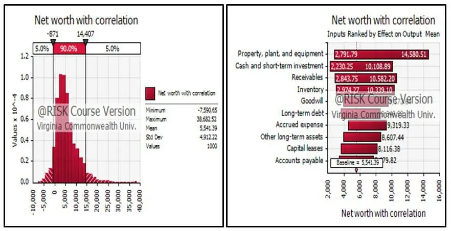 Figure 1: Value at Risk (VaR) of Amazon net-worth with correlation among the inputs
The quarterly data showed a probability of getting negative net worth at 5% value at risk, with ‘Property, plant, and equipment,’ and ‘Cash and short-term investments’ as the highest influencers of net worth. “So as far as the net worth goes,” says Dr. Baranoff, “Amazon is a strong company.” She also adds, “Interestingly the statistical distributions used for these inputs are Exponential distribution for net ‘Property, plant, and equipment,’ and ExtraValue distribution for ‘Cash and short term investments.’” These are shown in the following two graphs.
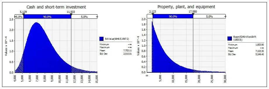 Figure 2: Amazon: Examples of statistical distributions for inputs
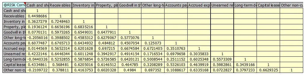 Table 1: Correlation among the applicable inputs for Amazon’s net-worth
 Figure 3: Sensitivity Analysis for Amazon net-worth with correlation among the inputs
Verifying the VaR results, the sensitivity analysis shows the relationship of the contribution of each of the inputs to the net worth. Again, as expected, ‘Property, plant, and equipment’ have the steepest slope. (As base value changes, ‘Property, plant, and equipment’ will have the biggest impact on net worth.)
 Figure 4: Stress Test for Amazon net-worth with correlation among the inputs
For the stress test4 it appears again that the ‘Property, plant, and equipment’ can stress Amazon’s net worth at the 5% VaR level.
While it is not shown here, the project also includes an examination of the inputs impacting the net income.
When the project begins, the students create a qualitative Risk Map for the company. Figure 5 is the Risk Map for Amazon. This is done independently from the @RISK analysis. The students study the company in depth using the 10K including all the risk elements faced by the company. They create a risk map based on qualitative data of ranking the risks by frequency and severity of the potential losses from the risk exposures. After they complete the @RISK analysis, they compare the results for the net worth and net income with the qualitative Risk Map’s inputs.
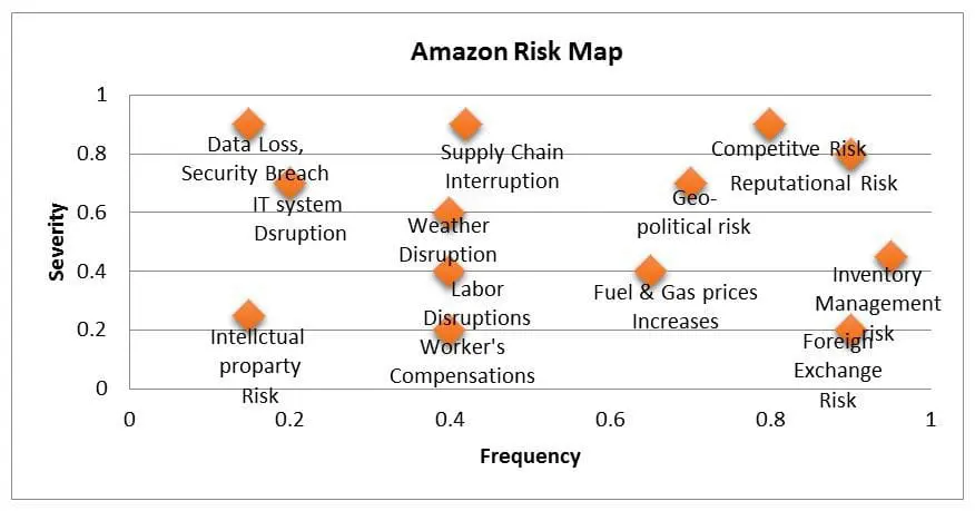 Figure 5: Risk Map for Amazon – Qualitative Analysis based on 10K Report
The @RISK analysis revealed that ‘Property, plant and equipment’ have the highest possibility to destroy the net worth of Amazon. In terms of the qualitative risk map, the connection would be to the risk of ‘Supply Chain Interruption.’ Any problems with plants’ equipment will lead to supply chain risk. Another connecting input is ‘Goodwill’ as a proxy for ‘Reputational Risk’ in the Risk Map. While it is high severity and high frequency by the students’ qualitative analysis, it is shown to have medium impact on the net worth of Amazon as per Figure 1 for the VaR analysis. Similarly, ’Goodwill’ has impact on the stress analysis in Figure 4, but, not as high as implied from the Risk Map.
For this short article, Dr. Baranoff has not discussed all the analyses done with @RISK and all the relationship to risks (inputs) in the Risk Map. Dr. Baranoff says they were able to draw conclusions about how Amazon should plan for the future: “In order to have high sales revenue, Amazon will need to maintain an excellent reputation and stay at competitive prices to avoid reputational risk and decline in market share,” she says. “Also, to avoid weather disruption risk and supply chain interruption risk, Amazon will need to diversify the locations of its properties and keep the warehouses spread across the country.”
Insurance and Finance, Virginia Commonwealth University
Analyzing FedEx
Dr. Baranoff’s students also analyzed the risk factors of FedEx, with the same objectives as for Amazon. The students gathered financial data from S&P Capital IQ, as well as from the FedEx investor relations website. With the information in hand, the students used @RISK for distribution fitting, stress analysis, and sensitivity analysis.
When analyzing FedEx’s risk factors, the students used the 10K of FedEx and then related them to the quantitative analysis using @RISK. A number of key areas came up, including Market risk, Reputational risk, Information Technology risk, Commodity risk, Projection risk, Competition risk, Acquisition risk, and Regulatory risk. The students created a risk map of all the factors, identifying the severity and frequency of each as shown in Table 6.
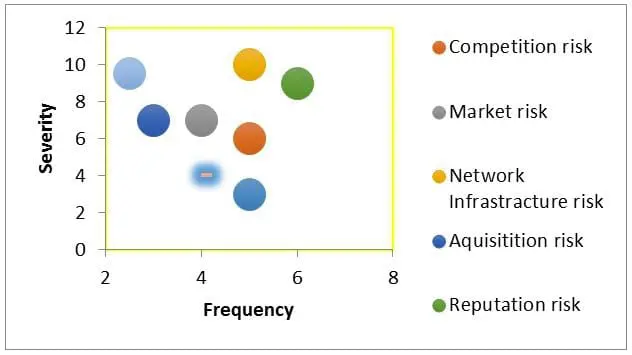 Figure 6: Risk Map for FedEx – Qualitative Analysis based on 10K Report
Working with @RISK for FedEx
The distribution fitting for most of the inputs on the FedEx income statement came up as a uniform distribution. This made sense to the students based on data from the last ten years, as FedEx has been a mature company strategically placing itself to confront changing market conditions. Net income was negative at the 45% VaR for the uncorrelated data against a 40% VaR for the correlated data. ‘Revenue’ and ‘Cost of goods sold’ are the two major contributors on net income.
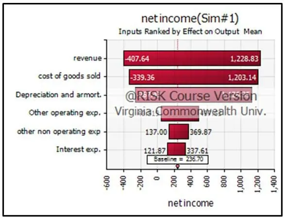 Figure 7: Value at Risk (VaR) for FedEx net-income with correlation among the inputs
The sensitivity analysis also confirms that ‘Revenue’ and ‘Cost of goods sold’ have the most influence. They are very large amounts compared to the other inputs on the income statement.
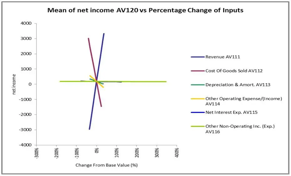 Figure 8: Sensitivity Analysis for FedEx net-income with correlation among the inputs
For the net worth, once again the most common distribution was the uniform distribution though there were a couple of normal distributions. Pensions had a lognormal distribution which is one of the most common distributions used by actuaries. Running the simulation with and without correlation had ‘Property Plant and Equipment’ (PPE) as the most influential input, but when running the simulation on the correlated balance sheet things evened out to a point where almost all the inputs had equal effects on net worth.
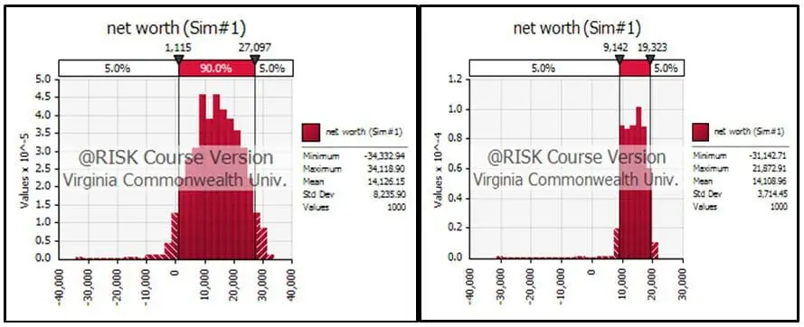
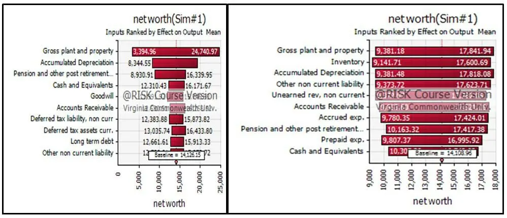 Figure 9: Value at Risk (VaR) for FedEx net-worth with correlation and without correlation among the inputs - Figures on left with correlation. Figures on right without correlation.
FedEx Segments
FedEx Corporation has 8 operating companies (FedEx Express, FedEx Ground, FedEx Freight, FedEx Office, FedEx Custom Critical, FedEx Trade Networks, FedEx Supply Chain, and FedEx Services). Since FedEx started with FedEx Express and acquired the rest of the operating companies for the segments, the data for FedEx Custom Critical, FedEx Office, FedEx Trade Networks, FedEx Supply Chain, and FedEx Services are reported in FedEx Express. The segments used by the students are therefore made up of FedEx Express, FedEx Ground and FedEx Freight. With that said, FedEx Express was the highest earner for the segments. FedEx Express had the lowest profit margin followed by freight and then ground. Where freight and ground only operate vehicles, Express operates aircraft as well, so it is logical that their expenses are higher as aircraft operations are much more expensive than vehicles. For segments without correlation, operating profit was negative all the way to the 25% VaR, but segments with correlation had positive operating profit at the 5% VaR. Also, the ranking of the inputs by effects for the segments were different for the correlated and uncorrelated inputs (see Figure 10).
Figure 10: Value at Risk (VaR) for FedEx Operating Profits with correlation
For the stress test analysis of the inputs impacting the output at the 5% VAR level, there wasn’t much of a difference between the correlated and uncorrelated segments even though the deviations from the baseline was more pronounced for the correlated than the uncorrelated segments, as can be seen in Figure 11.
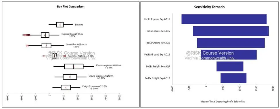 Figure 11: Stress Test for FedEx Operation Profits with correlation among the segments' inputs
The students concluded, “FedEx has strategically diversified itself to compete effectively in the global market place...Property Plant and Equipment was a big influence on net worth, but the company is constantly evaluating and adjusting this factor, so that there are no shortages or excesses.”
For Dr. Baranoff, @RISK’s ease of use is a major reason for making it the tool of choice for her classroom. Additionally, she lists its ability to provide credible statistical distributions as another major plus. “@RISK also allows me to show students the differences of selecting different statistical distributions, and the importance of correlation among some of the inputs,” she says. “Additionally, it allows us to combine the results for VaR analysis, stress analysis, and sensitivity analysis to discover what inputs can be destructive to a company’s net income and net worth. And, at the end of the day, it gives us good viewpoints to compare the results among the cases. The stories and the results lead to debate, and provide lots of fun in the classroom as the whole class become a risk committee.”
To conduct the comparison and give the tools to the risk committee to debate the risks and ways to mitigate them, the class creates Table 2.7 Table 2 is the foundation for the risk committee work. Each group is asked to provide a comparative evaluation among the cases under study (usually, about 5 cases each semester) as the second part of its case study report. This project concludes the semester.
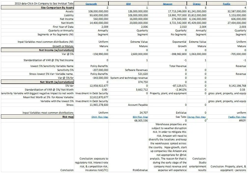 Table 2: Comparing all case studies for the Fall 2014 semester - Managing Financial Risk Course
Footnotes
1 Students first gathered financial statements from financial information provider S&P Capital IQ. 2 Each group attempts to have as many historical data points as possible to generate the statistical distributions. If quarterly data is available, it is used. The minimum number of observations cannot be less than 9 data points. 3 While “Accounts payable” are large in size, the input is no longer the most important variable under the correlation. As shown in Figure 1, it went to the bottom of the tornado. 4 The Stress test that is captured in the graphic takes the individual distributions that are fitted based on historical data, and stresses each inputs distribution for values that are within a specified range. In this example the range tested is the bottom 5% of the variables distribution. The goal is to measure each variable’s individual impact to an output variable when stressed. The box plots observe each stressed variable’s impact to the net worth (Assets-Liabilities) of Amazon. This test shows which variables distribution’s tails have the biggest ability to negatively or positive affect the company’s net worth at the tail of 5% value at risk net worth. Each variable is stressed in isolation, leaving the rest of the variables distributions untouched when determining the net worth values. When Assets are tested at their bottom 5% of their range, the net worth of the company is found to decrease as the distribution will be focusing on the bottom 5% of the distribution’s range resulting in less assets on the balance sheet. Likewise, when testing the bottom 5% of the liabilities, the distribution is focusing on small values for the liabilities, and due to the decrease in liabilities, net worth will increase when compared to the baseline run. 5 Each group creates its own version of the risk map as one template is not required. 6 See footnote 4. 7 We acknowledge some imperfections in Table 2, but it serves its purpose as a stimulating starting point for dialogue. 8 The students deserve recognition for their excellent work on the case studies presented in the matrix below. They are: Agack, Adega L., Alhashim, Hashim M., Baxter, Brandon G. Coplan, Thomas P., Couts, Claybourne A., Gabbrielli, Jason A., Ismailova, Railya K., Liu, Jie Chieh, Moumouni, As-Sabour A., Sarquah, Samuel, Togger, Joshua R.
Originally published: Oct. 28, 2022


