What is Monte Carlo simulation?
Monte Carlo simulation is a computational technique that uses repeated random sampling to model the probability of different outcomes in systems affected by uncertainty. Rather than producing a single estimated answer, it produces a distribution of possible answers, each with an associated probability. This lets decision-makers see the full range of what could happen, not just the most likely outcome.
How Monte Carlo simulation got its name
The Monte Carlo method as we know it today was developed in the 1940s by two scientists who were working on the Manhattan Project at Los Alamos National Laboratory: Stanislaw Ulam and John von Neumann. Ulam had to take some time off to recover from an illness. As he did so, he played many games of solitaire. He began to wonder whether it was possible to calculate the odds of whether a given deck would result in a win. This led to him thinking about whether random trials could solve problems too complex to compute directly.
Working with von Neumann, Ulam refined the technique to use in nuclear research. The method was named after Monte Carlo, the famous casino town in Monaco, because it relies on random chance, just like a deck of cards or a roulette wheel.
Monte Carlo simulation vs. the Monte Carlo method: What’s the difference?
The terms “Monte Carlo simulation” and “Monte Carlo method” are often used interchangeably, but they are not identical.
The Monte Carlo method refers to the broader class of probabilistic computational techniques that rely on repeated random sampling, which includes those used in pure mathematics and physics.
Monte Carlo simulation generally refers to the application of the Monte Carlo method for modeling complex real-world systems.
How does Monte Carlo simulation work?
Monte Carlo simulation works by representing uncertain inputs as probability distributions instead of fixed values. Simulations are run using a random number generator that draws a sample from each input distribution. This is repeated hundreds or thousands of times using randomly sampled values for each input.
Each iteration of the simulation represents one possible outcome. The collected results of these simulations show reveal the full range and probability of outcomes the system can produce: which outcomes are most likely, which are least likely, and which inputs account for the most risk.
For example, when estimating the cost of a construction project, you would define a range of values for your labor cost, material cost, and timeline instead of a single estimate. You would then set up a Monte Carlo simulation to run thousands of times, each time drawing a different random value from each range. This produces a probability curve showing how likely you are to come in over or under budget.
A simple Monte Carlo simulation example: rolling two dice
One common illustration of how Monte Carlo logic works is rolling two six-sided dice. As this explanation from Georgia State University demonstrates, there are 36 possible combinations. It is possible to compute the probability of each total exactly. This table shows the results:
Because this is a relatively simple system, it is possible to compute these probabilities by hand. However, you can also simulate 10,000 rolls of two dice and arrive at a similar distribution of probability. That is Monte Carlo simulation in miniature: when a system is too complex to compute manually, repeated random sampling produces the distribution.
How many simulations does it take to produce a good result with Monte Carlo methods?
The number of simulation runs needed to produce a good result with Monte Carlo methods depends on the complexity of the system being modeled. Most Monte Carlo simulations use between 1,000 and 10,000 iterations.
More iterations produce more accurate results because the output distribution stabilizes: as the sample size increases, confidence bounds on the result narrow. Very volatile or complex models may only converge after tens of thousands of iterations. Simpler models often produce stable results below 5,000 iterations. For most practical work, 5,000 iterations is a good default to start with.
What are the main components of a Monte Carlo simulation?
There are three main components of a Monte Carlo simulation:
- Input variables expressed as probability distributions
- A mathematical model that connects inputs to outputs
- Output variables, which are also expressed as probability distributions
Understanding each of the three components is crucial for creating a model that produces useful insights rather than noise.
Input variables
Input variables are the factors that influence the outcomes of the system you are measuring. The input variables for the construction project referred to earlier, for example, could include:
- Material costs
- Labor costs
- Energy costs
- Time to completion
Each of these variables should be defined as a probabilistic range rather than a single-point estimate. For example, “time to completion” would not be expressed as “six months”. Instead, it could be expressed as a triangular distribution with:
- A minimum time to completion of four months
- A most likely value of six months
- A maximum of 10 months
The distribution should be based on historical data if possible. If not, expert judgement can be used to develop a consensus.
The mathematical model
The mathematical model in a Monte Carlo simulation is the equation or set of relationships that connects inputs and outputs. A simple example would be:
Profit = Revenue – Expenses
The model itself does not change between simulations. Instead, what changes is the input values being fed into it. These input values are random samples from within the probability distribution.
Output variables
The outputs of a Monte Carlo simulation are also expressed as probability distributions rather than a single number. Instead of “the project will cost $1.2 million,” a Monte Carlo simulation output will look more like “there is a 70 percent probability that the project will come in within budget,” or “there is a 10% chance cost will exceed $1.5 million.”
Types of probability distributions in Monte Carlo simulation
The four probability distributions most used in Monte Carlo modeling are normal, triangular, uniform, and lognormal. Each distribution is suited to a different kind of uncertainty.
The probability outputs you select for your inputs will determine how realistic the outcomes of your simulation are.
Normal distribution (bell curve)
The normal distribution is symmetrical and bell-shaped. It is defined by a mean and a standard deviation. It is used when values cluster around an average, with large deviations becoming progressively less likely.
Common examples of normal distribution include manufacturing tolerances, standardized test scores, and measurement errors. The example of rolling two six-sided dice given above also fits a normal distribution.
Triangular distribution
The triangular distribution is defined by three values: minimum, most likely, and maximum. It is common in project management and business forecasting, where experts can usually estimate a plausible range and most likely value, but lack the data for a more precise distribution.
Uniform distribution
In a uniform distribution, every value within a defined range has equal probability. It is appropriate where there is genuine uncertainty across a range with no preferred outcome. The outcome of rolling a single six-sided die, for example, would have a uniform distribution.
Lognormal distribution
The lognormal distribution is right-skewed and always has positive values. It is common in finance, particularly in stock prices and option pricing How to run a Monte Carlo simulation: a step-by-step guide
Running a Monte Carlo simulation follows the same process regardless of whether you are modeling a financial portfolio, a project schedule, or a manufacturing line.
Step 1: Define the problem and identify the output variable
Decide what you are trying to model and what success or failure looks like. The output variable—the project completion date, total cost, or portfolio return—must be defined before any modeling work begins. Vague outputs produce vague results.
Step 2: Identify all uncertain input variables
List every input that has a meaningful level of uncertainty. Avoid the temptation to fix inputs that feel “close enough.” Because simulations involve thousands of iterations, even small errors in defining input variables can result in large errors in outputs.
Step 3: Assign probability distributions to each input
Choose the distribution type (normal, triangular, uniform, or lognormal) that best fits each input variable. Collect relevant historical data or request expert judgement to clearly identify the behaviors of the different input variables.
This is one of the most consequential steps in the entire process. Your output will depend on the quality of your data. Remember: garbage in, garbage out.
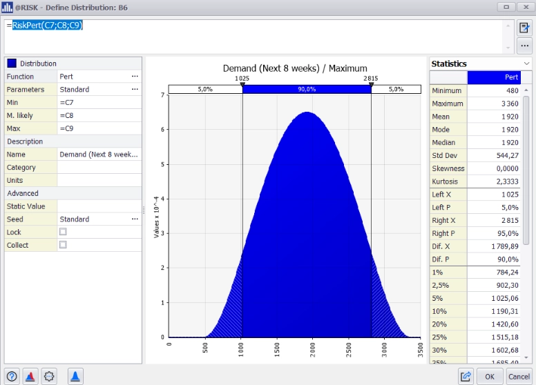
@RISK Monte Carlo simulation model of demand using the Pert distribution function.
This is one of the most consequential steps in the entire process. Your output will depend on the quality of your data. Remember: garbage in, garbage out.
Step 4: Build the mathematical model
Connect inputs to output through a formula or model. This may be as simple as Profit = Revenue − Expenses, or as complex as a multi-variable project schedule with interdependencies. The structure of the model does not change between simulations: only the input values do.
Step 5: Run the simulation
The software will randomly sample values from each input and plug them into the model, generating however many iterations you define—typically 1,000 to 10,000 times. Each iteration represents one outcome. Together, the iterations will produce a distribution of outcomes that capture the system’s range of behavior.
Step 6: Analyze the output distribution and run sensitivity analysis
Examine the output histogram. What is the probability of hitting your target? Which range covers 80 percent of outcomes? Then run a sensitivity analysis (also known as a tornado analysis due to the shape of the graph it produces) to identify which inputs drive the most variability in the output. This shows you where to focus your risk management efforts.
Monte Carlo simulation software like @RISK by Lumivero make it possible to complete each step of the Monte Carlo simulation process—from distribution fitting to creating sensitivity charts—from within Excel. To see an example of how this workflow can be built out, read about how to run a Monte Carlo simulation in Excel.
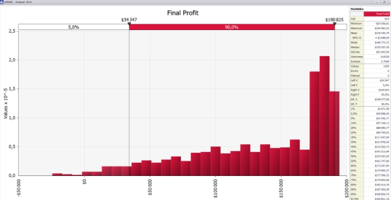
Final profit graph in @RISK showing the likelihood of all scenarios.
What are some common use cases for Monte Carlo simulation?
Monte Carlo simulation can be used wherever decisions depend on uncertain inputs—and where the cost of being wrong comes with high stakes. The technique can be applied across industries, but several fields lean on it more than others.
Finance and investment
Finance and investment applications of Monte Carlo simulation include:
- Portfolio risk modeling
- Value at Risk (VaR) calculations
- Options pricing
- Retirement and long-term return projections
- Stress-testing different regulatory frameworks
Single-point forecasts cannot capture the range of market outcomes, which is why Monte Carlo simulation is a key part of the analytical toolkit in qualitative finance.
Project management and scheduling
Project managers use Monte Carlo for cost estimation and for modeling schedule risk. Distributions are assigned to task durations and dependencies, and the full schedule is simulated to produce a probability curve for completion.
Compared to a single estimated end date, outputs from Monte Carlo simulation produce a more reliable indication of how likely it is the project will finish on schedule.
Engineering and reliability testing
Engineers apply Monte Carlo simulation to forecast product failure rates, structural reliability, and system durability. Rather than testing designs at nominal values, Monte Carlo simulation helps engineers simulate performance across the full distribution of tolerances, loads, and environments.
This produces a result that gives a probability for the design meeting requirements rather than a simplistic pass/fail outcome.
Manufacturing and supply chain management
Monte Carlo simulation helps manufacturers and supply chain planners cope with demand uncertainty, lead time variability, and supplier risk. Inventory and production schedules can be evaluated against a range of demand rooted in historical data or expert analysis rather than an average.
This allows for plans that are resilient enough to handle disruption beyond expected conditions.
Business analytics and forecasting
Business analysts use Monte Carlo simulation for:
- Revenue forecasting
- Pricing models
- Marketing ROI estimates
- New product launch planning
Wherever a forecast depends on multiple uncertain inputs, from conversion rate to price elasticity, running a Monte Carlo simulation produces a more workable outcome than a single number that is likely to be wrong in some direction.
Healthcare and pharmaceuticals
Healthcare and pharmaceutical organizations apply Monte Carlo simulation to clinical trial design, resource allocation, and even for planning regulatory submissions.
Uncertain inputs such as trial enrollment rates, dropout rates, and effect sizes can all benefit from probabilistic modeling rather than fixed assumptions.
Sports analytics and tournament forecasting
Monte Carlo simulation is widely used in sports analytics to estimate the probability of different outcomes in games, tournaments, and entire seasons. By simulating thousands of possible scenarios based on team performance metrics, historical data, and other variables, analysts can move beyond simple predictions to understand the full range of potential outcomes and their likelihood.
For example, Monte Carlo simulation can be used to estimate a team's chances of winning the World Cup, predict outcomes for March Madness tournament brackets, or build probabilistic models for the Super Bowl. Rather than relying on a single forecast, decision-makers can evaluate the probability of reaching different stages of a tournament, advancing through playoff rounds, or ultimately winning a championship.
This approach helps teams, broadcasters, sports bettors, and fans better understand uncertainty and make more informed decisions based on probabilities rather than assumptions.
See real-world examples of Monte Carlo simulation in action.
Advantages of Monte Carlo simulation
Compared to deterministic forecasting and scenario analysis, Monte Carlo simulation has five core advantages:
- Monte Carlo simulation can handle complex, non-linear systems, making it possible to model multiple interacting variables simultaneously.
- Monte Carlo simulation models a full probabilistic distribution of results—not just best, worst, and average.
- Monte Carlo simulation enables sensitivity analysis by identifying which inputs have the greatest impact on the output.
- Monte Carlo simulation can scale with complexity, because accuracy improves as more iterations are run.
- Monte Carlo simulation results in more actionable insights. “There is a 70 percent probability of completing on time” is more useful to decision-makers than “we estimate the project will take six months.”
In practical terms, these advantages translate into more nuanced and confident decisions. Rather than presenting a forecast that hides its assumptions inside a single number, a Monte Carlo output puts the assumptions on the table and shows a range of plausible answers. Sensitivity analysis turns that into action: it points to the inputs that drive the greatest variability, helping decision-makers develop targeted mitigation strategies.
Disadvantages and limitations of Monte Carlo simulation
Monte Carlo simulation requires careful implementation and may not be useful for modeling every type of system. Potential disadvantages may include:
- Monte Carlo simulation results depend entirely on input quality. A lack of data or a poorly chosen distribution will produce misleading outputs for any number of iterations.
- Monte Carlo simulation may require significant computing infrastructure, power, or time to run if models are sufficiently complex.
- Monte Carlo simulation requires expertise for effective set up, including domain knowledge to inform appropriate selection of probability distributions for input variables or to produce usable historical data.
- Monte Carlo simulation results may not converge when modeling highly volatile systems, even after tens of thousands of iterations.
- Monte Carlo simulation results may underestimate the probability of extreme events (sometimes called “fat tails”) in financial or systemic risk scenarios when using standard distributions.
The first limitation is the most important. Remember, a Monte Carlo simulation does not generate information. Instead, it propagates the information you give it through a model. If the input distributions are wrong, the output distribution is wrong, and thousands of iterations only make the wrong answer look more authoritative.
This is why any serious Monte Carlo workflow requires close attention to distribution fitting and validation. It’s also why purpose-built tools for Monte Carlo simulation include automated distribution-fitting features.
Monte Carlo simulation vs. deterministic analysis
Deterministic models are those that take fixed input values and produce a single output as a result. A deterministic model can be useful when inputs are known and uncertainty is low. In any system affected by uncertainty, however, Monte Carlo simulation offers a better solution. It produces probability statements rather than a single estimate.
Neither approach is wrong in absolute terms—they answer different types of questions. When in doubt, if a decision depends on uncertain inputs, Monte Carlo is a more honest tool.
Monte Carlo simulation and AI
AI is removing the friction that has always kept practitioners from using Monte Carlo well, and AI tools help accelerate parts of the Monte Carlo simulation workflow that traditionally require significant time from experts. Machine learning models, for example, can reduce the time spent on distribution fitting by making recommendations based on historical input data. Large language models can lower the barrier for non-modelers by translating plain-language descriptions of processes into structured model inputs.
AI is also being used to surface overlooked risk factors by analyzing patterns from past simulation outputs. It is also helping to automate parts of sensitivity analysis without manual interpretation, such as flagging inputs that need closer attention.
None of these applications of AI will replace the underlying Monte Carlo method or remove the need for expert insight into data selection and modeling. Instead, they help make models faster to set up. For a practical guide, see our full article on using AI with Monte Carlo simulation.
Run Monte Carlo simulation inside Excel with @RISK
Monte Carlo simulation becomes even more powerful when you don’t have to build your model from scratch. @RISK by Lumivero is a Monte Carlo simulation software add-on for Microsoft Excel that allows you to handle distribution fitting, simulation runs, and sensitivity analysis from inside the spreadsheet environment your team already uses.
Wherever probabilistic decision-making is needed—in finance, project management, engineering, and pharmaceutical research—@RISK can help create actionable insights.
Make uncertainty work for you
Unlock the power of probabilistic modeling without having to start from square one. Bring a full suite of powerful tools for Monte Carlo simulation—from distribution fitting to board room-ready reporting—right into Microsoft Excel with @RISK by Lumivero.